7.3. Sampling Linear Scale-Space
Most of what we have done in the chapter up to now has been formulated for images in the continuous domain. And it is due to our use of the Gaussian derivatives that this is even true for everything involving derivatives. In practice working with discrete (i.e. sampled images), when using the simple strategy of discretizing the convolution operation by sampling the kernel function as well, we are doing ok in case the scale of the Gaussian filter involved in the Gaussian derivative is greater than ome.
So we are used to deal with sampled images in practice. Sampling an image in the spatial domain is invariably done using a regular, most often square, grid of sample points. But what about sampling a scale space? Let \(F^{s_0}\) be the sampled version of the image we start with in constructing a scale space, i.e.
then the image \(F^s\) at scale \(s\) is calculated from \(F^{s_0}\) as:
To store and process the scale space we have to decide for which scales \(s\) to calculate and store the convolutions. You might be tempted to use a equidistant sampling of the scale as well. But that would require a dense sampling of the scale and because scale tends to be of interest over several orders of magnitude (scales ranging from tenths to hundreds are not uncommon) that would require a tremendous number of scales to process. And it is not needed. You can try it for yourself and for instance compare images at scale \(s=1\) and \(s=2\). The increase in scale is quite noticable in that case. But comparing \(s=100\) with \(s=101\) shows hardly any difference at all. It is better to sample scale equidistantly on a logarithmic scale axis.
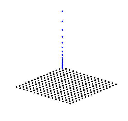
Fig. 7.7 Sampling Scale Space. To avoid visual clutter we have only shown the sample points in space for scale \(s_0\) and the scale samples for \(\v k=\v 0\).
The scale in scale space is sampled logarithmically. If \(s_0\) is the first scale (often the scale of the image that was obtained with a camera) then the scales are:
for \(i=0,\ldots,\nscales-1\) where \(\smax=s_{\nscales-1} = \alpha^{\nscales-1} s_0\) defines the maximal scale we are interested in. The constant \(\alpha\) defines the (multiplicative) step size along the scale axis.
As a rule of thumb the scale factor \(\alpha\) should be somewhere in the region \(1<\alpha\leq2\). With the extreme value \(\alpha=2\) the scale doubles with every scale sample. Although that is nice from a computational point of view (see the subsection on Burt pyramids) we often opt for a smaller \(\alpha\) in order not to miss important features in scale space (e.g. when looking for the exact localization of blobs in scale space).
7.3.1. Direct versus Incremental Calculation
Let our goal be to make a scale scape from initial image \(F^{s_0}\) where where take \(s_0=0.5\). In that case the receptive fields of the samples just overlap. Let the largest scale we want to represent in the scale space be \(s_\text{max}\) and we wish to have \(n_\text{scales}\) scales starting at \(s_0\) and ending at \(s_S=s_\text{max}\) then the \(\alpha\) value follows from that:
The images \(F^{s_i}\) are calculated as:
for \(i=1,\ldots,\nscales-1\). Note that \(F^{s_0}\) is the original image and needs no convolution. We will call this the direct calculation of the scale space.
Show code for figure
 1import numpy as np
 2import matplotlib.pyplot as plt
 3from scipy.ndimage import gaussian_filter as gD
 4
 5
 6def make_scale_space_direct(f, s_0, s_max, n_scales):
 7    alpha = (s_max / s_0)**(1 / (n_scales - 1))
 8    scales = s_0 * alpha**np.arange(n_scales)
 9    diff_scales_from_s0 = np.sqrt(scales[1:]**2 - s_0**2)
10
11    fs = np.empty((n_scales, *f.shape))
12    fs[0] = f.copy()
13
14    for i, s in enumerate(diff_scales_from_s0):
15        fs[i + 1] = gD(f, s)
16
17    return fs, scales
18
19
20def make_scale_space_incremental(f, s_0, s_max, n_scales):
21    alpha = (s_max / s_0)**(1 / (n_scales - 1))
22    scales = s_0 * alpha**np.arange(n_scales)
23    diff_scales_from_si = np.sqrt(scales[1:]**2 - scales[:-1]**2)
24
25    fs = np.empty((n_scales, *f.shape))
26    fs[0] = f.copy()
27
28    for i, s in enumerate(diff_scales_from_si):
29        fs[i + 1] = gD(fs[i], s)
30
31    return fs, scales
32
33
34def make_scale_space_octaves(f, O, k, s0):
35    n = O * k
36    alpha = 2 ** (1 / k)
37    scales = s0 * alpha ** np.arange(n)
38    conv_scales_from_s0 = s0 * np.sqrt(alpha ** (2 * np.arange(n)) - 1)
39
40    fs = np.empty((n, *f.shape))
41    fs[0] = f.copy()
42
43    for i, s in enumerate(conv_scales_from_s0[1:]):
44        fs[i + 1] = gD(f, s)
45
46    return fs, scales
47
48
49plt.close('all')
50
51try:
52    f = plt.imread('../../source/images/voc21.jpg')
53except FileNotFoundError:
54    f = plt.imread('source/images/voc21.jpg')
55
56g = f[38:348, 156:400, 1] / 255
57
58n_scales = 8
59s0 = 0.5
60s_max = 32
61fs_direct, scales = make_scale_space_direct(g, s0, s_max, n_scales)
62
63fig_scsp_direct, axs = plt.subplots(1, n_scales, figsize=(n_scales, 2))
64n = n_scales
65
66for i, s in enumerate(scales):
67    axs[i].imshow(fs_direct[i], cmap=plt.cm.gray)
68    axs[i].axis('off')
69    axs[i].set_title(f"{s:2.2f}")
70
71    plt.tight_layout()
72
73
74fs_incremental, scales = make_scale_space_incremental(g, s0, s_max, n_scales)
75
76fig_scsp_incremental, axs = plt.subplots(2, n_scales, figsize=(n_scales, 4))
77n = n_scales
78
79for i, s in enumerate(scales):
80    axs[0, i].imshow(fs_incremental[i], cmap=plt.cm.gray)
81    axs[0, i].axis('off')
82    axs[0, i].set_title(f"{s:2.2f}")
83
84    axs[1, i].imshow(fs_direct[i]-fs_incremental[i], cmap=plt.cm.gray)
85    axs[1, i].axis('off')
86    axs[1, i].set_title(f"{(np.abs(fs_direct[i]-fs_incremental[i])).max():2.1E}")
87    plt.tight_layout()
88fig_scsp_direct.savefig('source/images/scsp_voc21.png')
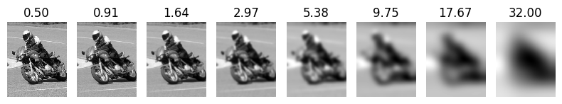
Fig. 7.8 Direct calculation of a scale space. All scales \(s>s_0=0.5\) are calculated as \(F^{s_0} \star G^{s_0 \sqrt{\alpha^{2i}-1}}\). The scale \(s_i\) is printed above the images.
Instead of the direct calculation of scale space we may take the image at scale \(s_i\) to calculate the image at scale \(s_{i+1}\):
This is called the incremental calculation of scale space. The advantage is that incremental calculation is more efficient (faster) as the scales in convolutions are smaller. A disadvantage is that the Gaussian convolution is less accurate for smaller scales. As a rule of thumb we do need a scale for the convolution kernel greater than around 0.7.
Show code for figure
1# for code see previous figure
2fig_scsp_incremental.savefig('source/images/scsp_voc21_incremental.png')
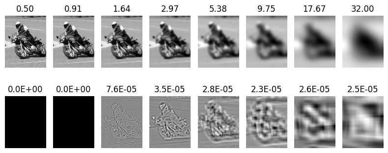
Fig. 7.9 Incremental calculation of a scale space. In the first row the scale space images calculated incrementally. On the second row the difference images for all scales are shown (note that the very small differences are displayes over the entire dynamic range of the display, and therefore look larger than they are). In the first row the scale is printed at the top of an image, In the bottom row the maximal absulte difference of the images at scale \(s_i\) calculated directly and incrementally.
From the figure it is clear that the differences are very (neglibly) small. So where possible an incremental calculation is called for. Note that in case we are calculating the scale space of a derivative we must be more careful.
7.3.2. Pyramids
When constructing a scale space we are smoothing images. After smoothing an image we need less pixels to represent the image faithfully. The exact understanding of this fact requires knowledge of the sampling theorem which falls outside the scope of this lecture series. But you can imagine that when we smooth out local variations in an image we can subsample the image without loosing too much information.
As a rule of thumb, which is useable when using Gaussian smoothing, we may subsample an image with a factor of 2 (in both directions) when the scale of smoothing has doubled.
Fig. 7.10 Subsampling Images WITHOUT Smoothing.